Gamma Graph#
A two-parameter family of planar proximity graphs based on gamma-neighborhood emptiness (Veltkamp, 1992).
An undirected edge between two sites \(p\) and \(q\) is included when a parameterized neighborhood region around segment \(pq\) contains at most \(k\) other points.
Constructor#
Gamma_Graph(setpoints, gamma0=0.0, gamma1=0.0, k=0, closed=True, block_size=1000)
Parameters:
setpoints (SetPoints): The set of points (must be 2D).
gamma0 (float): Radius/scale parameter (must satisfy \(-1 < \gamma_0 < 1\)).
gamma1 (float): Neighborhood composition parameter (must satisfy \(-1 < \gamma_1 < 1\)).
\(\gamma_1 \le 0\): neighborhood is an intersection of two discs.
\(\gamma_1 > 0\): neighborhood is a union of two discs.
k (int): Allowed number of other points inside the neighborhood (must satisfy \(k \ge 0\)).
closed (bool): If True, uses \(\le\) (closed discs). If False, uses \(<\) (open discs).
block_size (int): Batch size for vectorized point-in-neighborhood counting.
Mathematical Definition:#
Let \(P = \{p_1,\dots,p_n\} \subset \mathbb{R}^2\) with Euclidean norm \(\|\cdot\|\). For two distinct sites \(p,q\in P\), define midpoint \(m = \tfrac{p+q}{2}\) and half-length \(r = \tfrac{\|p-q\|}{2}\).
For \(-1 < \gamma_0 < 1\), define the disc radius
and the perpendicular-bisector offset
Let \(n\) be a unit normal to the direction \(q-p\) (two choices: \(\pm n\)). Define the two disc centers on the perpendicular bisector:
Let \(D(c,R)\) denote either the closed disc \(\{x:\|x-c\|\le R\}\) if closed=True,
or the open disc \(\{x:\|x-c\|< R\}\) if closed=False.
Define the gamma-neighborhood
Define the interior count
Then \((p,q)\) is an edge iff
Special Cases (limits):
\(\gamma_0=\gamma_1=0\) with \(k=0\) reduces to the Gabriel Graph.
The boundary parameter values \(\pm 1\) correspond to half-space/degenerate neighborhoods in the original definition; here they are approached as limits because \(\gamma_0,\gamma_1\in(-1,1)\) are required.
Properties:
Increasing \(|\gamma_0|\) increases \(R\), enlarging the neighborhood and typically removes edges (stricter emptiness).
Switching from intersection (\(\gamma_1\le 0\)) to union (\(\gamma_1>0\)) enlarges the neighborhood and typically removes edges.
Increasing \(k\) typically adds edges, interpolating from an empty-neighborhood graph (\(k=0\)) to denser graphs.
Value Errors / Limitations:
Raises
NotImplementedErrorifsetpointsis not 2D.Raises
ValueErrorifgamma0orgamma1is not in \((-1,1)\).Raises
ValueErrorifk < 0.Raises
TypeErrorifkis not an integer or ifclosedis not boolean.Raises
TypeErrorifblock_sizeis not an integer or ifblock_size <= 0.
Example#
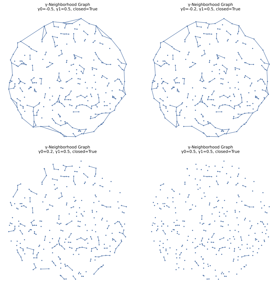
import proximitygraphs as pg

pts = pg.SetPoints.uniform_sphere(n=300, seed=7)  # unit disk (2D)

G1 = pg.Gamma_Graph(pts, gamma0=-0.5, gamma1=0.5, k=0, closed=True, block_size=128)
G2 = pg.Gamma_Graph(pts, gamma0=-0.2, gamma1=0.5, k=0, closed=True, block_size=128)
G3 = pg.Gamma_Graph(pts, gamma0=0.2, gamma1=0.5, k=0, closed=True, block_size=128)
G4 = pg.Gamma_Graph(pts, gamma0=0.5, gamma1=0.5, k=0, closed=True, block_size=128)

graphs = [G1, G2, G3, G4]
pg.draw_grid(graphs, 2, 2, figsize=(10, 10), details=True)
Reference#
Remco C. Veltkamp (1992). The gamma-neighborhood graph. Computational Geometry: Theory and Applications, 1, 227–246.